
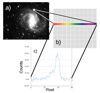
Figure 1 – How spectra are obtained by Gaia. The light from the target (a) is spread out in wavelength, making a spectrum (b). This spectrum is measured by a CCD, and the counts in each pixel are plotted on the Gaia Alerts web pages (c).
One of the unique capabilities of Gaia is that the satellite obtains a low resolution spectrum for every source it observes. You can read more about spectroscopy (Why we take spectroscopy), while below we give some background information to help you interpret the spectra shown on the Gaia Alerts web pages.
The first thing to note is that all the Gaia spectra shown here are uncalibrated, i.e. they are in their raw state. When Gaia observes a spectrum using the blue photometer (BP) and red photometer (BP) (see Blue and Red Photometers), it uses something similar to a prism to disperse the light from a star into different colours (see Fig. 1). This dispersed light falls onto the pixels in a charge coupled device (CCD) similar to that in a smartphone (Fig. 1b). Finally, the spectrum is plotted as the number of counts measured from the light in each pixel (Fig. 1c).
When an astronomer takes a spectrum of an object, they usually calibrate it, to convert the spectrum from an instrumental measurement of "counts per pixel" to a physical measurement of "intensity of light per wavelength". To do this, the astronomer needs to know exactly how sensitive the CCD is to light of a given wavelength, and how many pixels light of a given wavelength is spread over. For Gaia, a team at the Institute of Astronomy in Cambridge are calibrating all the observed spectra, but these will not be ready until later in the mission. But since we want to do science with Gaia Alerts right now, we can't wait for the calibrated spectra – hence we decided to show the uncalibrated spectra on our web pages.
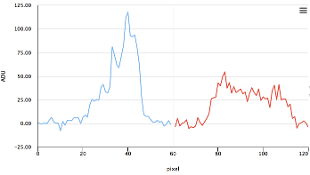
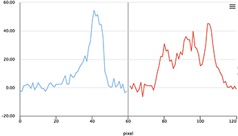
Figure 2 – An example of a spectrum from Gaia. The BP spectrum is from pixels 20 to 45, while the RP spectrum is from pixels 80 to 110.
The second key point to note is that Gaia takes low-resolution spectra of each object with the blue photometer (BP) and red photometer (BP). The BP covers wavelengths from 330 to 680 nm, while the RP covers 640 to 1050 nm. On the plots you will see on the Gaia Alerts pages, we show both BP and RP spectra on a single figure, with the former in blue, and the latter in red (Fig. 2). The wavelength and flux calibrations for BP and RP are slightly different, and so it is hard to compare them directly. However if an object has a higher peak counts in RP we generally say it is red, and probably cool (like an M-star, or an elliptical galaxy). Conversely, objects with a larger number of counts in BP are blue, and are probably hot sources such as young supernovae, cataclysmic variables, or quasars.
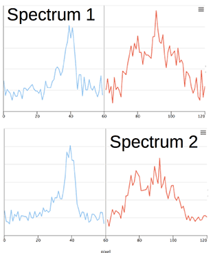
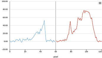
Figure 3 – Two consecutive spectra of a faint target. The small differences are due to low signal-to-noise, rather than astrophysical differences.
Many of the spectra seen by Gaia are of relatively faint objects. In particular, objects that are fainter than magnitude G=16 will have relatively low "signal-to-noise". What this means is that many of the bumps and peaks seen in the spectra are not due to the target, but rather are due to the fact that we only have a small amount of light to work with. In Fig. 3, you can see an example of two spectra, taken of the same object (Gaia15afh) when it was magnitude G=18.4. As these spectra were taken less than two hours from each other, the target should appear virtually identical in each. Instead, we see that while the main features of the two spectra are the same (the peak in the BP spectrum at pixel 40, and the peaks in RP at pixels 80 and 90), there are small pixel-to-pixel variations that are simply due to the low signal-to-noise. These small variations should hence be ignored when interpreting the spectra.
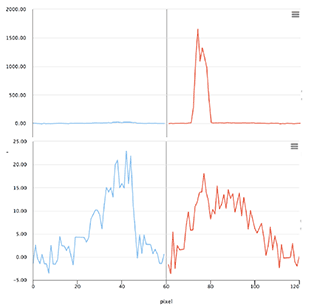
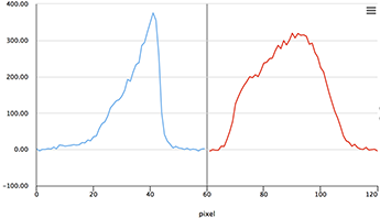
Figure 4 – An example of two spectra of the same object, where the first spectrum overlaps with an unrelated nearby source, leading to a large number of counts in RP.
Finally, there are occasionally other issues with the spectra. The most common problematic situation is where there is a nearby source that overlaps with the spectrum of the object we are interested in. In Fig. 4, we show two spectra of Gaia16anq, observed back to back. In the first spectrum, we see an extremely bright, red source – we only see the RP spectrum, and it has a peak of about 1500 counts. The high number of counts in the spectrum is inconsistent with the magnitude of the source (G=18.9). Moreover, in the second spectrum taken just over an hour later, we see that the counts are much lower (peaking at around 20), and that the source is seen in both the BP and RP spectra. What has happened, is that for the first spectrum, a nearby red star happened to overlap the spectrum of Gaia16anq on the CCD. The second spectrum was taken at a slightly different angle, and so the two objects did not overlap. As a general rule of thumb, if there are significant differences between two spectra of the same object, taken close together in time (within a few hours of each other), this is probably due to a problem with the data.
Examples
 Gaia16anx: This is a supernova, as can be seen from the broad peaks in the RP spectrum.
 Gaia16aoz: This is a nice example of a high signal-to-noise spectrum. The blue featureless spectrum is characteristic of something hot, such as either a quasar or a cataclysmic variable in outburst. In this case, the target was a known quasar.
 Gaia16aon: The spectrum is red, and has a very broad dip between pixels 80 and 90. This is caused by molecules present in the atmosphere of a very cool M-type star.